Let me start with a question.
Do you like solving Data Structure & Algorithms problems during interviews?
If you’re like me the answer is hell no. I hated doing it at my school. I hated doing it at university. And, surprise-surprise, I hate it now.
But here’s the deal – to get an awesome job you need to get good at solving coding problems. You just have to learn how to solve these abstract, out of real life challenges.

Unlike my more talented peers I never liked these problems. Instead of programming cool stuff like games I had to spend ungodly amount of time studying boring crap like segment trees that I hardly use anywhere.
However to succeed at an interview you have to learn at least basic algorithms and data structures. And one of problem solving techniques you’ll want to learn is called Dynamic Programming (aka DP).
DP seemed to give me the most trouble. I spent a good few years collecting nuggets of wisdom from here and there before it finally clicked with me.
In this blog post I hope to give you the same ‘aha’ moment. I hope to shine light on what DP is and how to use it.
Let’s start with the first major hurdle I have with DP.
Dynamic Programming is a terrible name
What do you think of when you hear ‘Dynamic Programming’?

I will confess – I had no idea what I was about to learn. It looks like we will, umm, program something that’s changing as we code it? I dunno ¯\_(ツ)_/¯.
It’s often said that there are 2 big problems in programming – cache invalidation and naming things. Looks like we have failed the latter problem here.
Let me give you an alternative name for DP – Brute Force with Caching. Since we all are well respected Computer Scientists here we must acronymify it – BFwC.

Alright, what does this mean?
Basically we solve our problem by recursive brute force. If our problem happens to have a nice structure we can split it into smaller sub-problems (this is the ‘dynamic’ part of the dynamic programming). We keep going down until we hit a trivial base case. We start going up solving sub-problems and in the process caching and reusing these solutions (that’s the ‘programming’ part of the dynamic programming). And magically instead of taking exponential time our brute force solution takes polynomial times aka much less time!
This is all nice and dandy but you’re probably still scratching your head. Let’s get our hands dirty with a simple problem. You might have heard about it before.
Let’s compute Fibonacci Sequence
I know, it’s not the most exciting or practical problem out there. But did you know that solution to this problem is actually a DP algorithm? Bear with me for a few minutes because we’re about to unearth some fundamental knowledge here.
In case you forgot Fibonacci Sequence looks like this:
0, 1, 1, 2, 3, 5, 8, 13, 21, 34, 55, 89, 144 …
You start with two numbers, 0 and 1. After that your next number is a sum of the previous 2 numbers.
Let’s define F[0] = 0, F[1] = 1. Then for i = 2, 3, 4 … F[i] = F[i-1] + F[i-2].
How can we compute the n-th Fibonacci number?
Well, one of the ways would be to use the definition directly:
int F(int n) {
    if (n == 0) return 0;
    if (n == 1) return 1;
    return F(n-1) + F(n-2);
}
We have successfully split our problem into sub-problems – to compute F[n] we compute F[n-1] and F[n-2] first.
Let’s say that we want to compute F[5]. That’s easy, F[5] = F[4] + F[3]. Okay, but what are F[4] and F[3]? Well, F[4] = F[3] + F[2] and F[3] = F[2] + F[1]. Great, but this is not an answer yet. Do we know what F[2] and F[1] are? Well, F[2] = F[1] + F[0]. But we do know what F[1] and F[0] are – they are 1 and 0 by definition!
Let’s expand F[5] as our computer would:
F[5]                              // expand F[5]=F[4]+F[3]
= F[4]+F[3]                       // expand F[4]=F[3]+F[2]
= (F[3]+F[2])+F[3]                // expand F[3]=F[2]+F[1]
= ((F[2]+ F[1])+F[2])+(F[2]+F[1]) // expand F[2]=F[1]+F[0]
= (((F[1]+F[0])+F[1])+(F[1]+F[0]))+((F[1]+F[0])+F[1])
= 1+0+1+1+0+1+0+1
= 5
Here’s a visual representation of what we’ve just discovered.

This is a dependency tree for Fibonacci numbers. To compute F[5] we need F[4] and F[3]. To compute F[4] we need F[3] and F[2] and so on. Can you see how our final result is the sum of just F[1] and F[0]?
This is a huge drawback in our approach. Can you see how we’re expanding F[3] 2 times and F[2] 3 times? Doesn’t that seem wasteful? Why not save F[4], F[3] and F[2] after we have computed them?
// we will cache our values into an array
// -1 means that we haven't computed this value yet
int fib[6] = {0, 1, -1, -1, -1, -1};

int F(int n) {
    // have we already computed this value before?
    if (fib[n] > 0) return fib[n];

    // if no, compute fib[n] using the definition and cache it
    fib[n] = F(n-1) + F(n-2);
    return fib[n];
}

// after calling F(5) fib will look like this:
// fib = {0, 1, 1, 2, 3, 5};

Here we compute F[2], F[3], F[4] and F[5] just once. We cache and reuse their values as needed. This means that we don’t expand our computation down to the base cases F[1] and F[0]. We have just truncated the number of computations by half!
Let’s take a step back and reiterate over what we’ve just accomplished. We have started with a recursive brute force solution – compute F[n-1] and F[n-2] and then add these values. We have noticed that we’re recomputing F[i] for i=1..n-1 many times all over again. That’s wasteful so we started saving values to an array. We have modified our code to lookup value in the array. If it’s there we take it, otherwise we compute the value and store it into the array.
Okay, now we’re ready for a more challenging problem. Don’t worry, it’s not that bad… yet 😉
Let’s climb some stairs
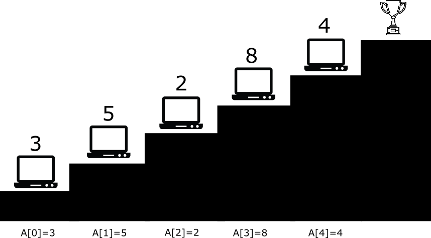
Here’s another fun practical problem for you. Let’s say that you want to climb a staircase. You can make 1 or 2 steps at a time. Every stair has a computer on it. To move to the next stair you need to solve A[n] coding problems. You can start from the 1st or the 2nd stair. Given array A what is the minimum number of problems you must solve to climb to the top of the Stairs of Fun?

I encourage you to solve the problem on picture by hand. Spoiler – the answer is nine.
Now that you’re back – how can we solve this problem for any staircase?
You might be tempted to take the best solution at each step and hope that it gives you the best global result. Here’s another staircase for you:

We start at stair 1 because otherwise we would solve 5 problems. Next we make a big step to the 3rd stair skipping 5 problems, than a small step to the 4th and then we reach the top. We must solve 3+4+1=8 problems.
This is called a greedy approach and sadly it doesn’t work here:

Here’s a better solution – if we start from the second stair we need to solve 5+1=6 problems. Moral of the story – don’t get too greedy solving coding problems 🙂
Where greediness fails DP prevails. So let’s try this DP thing.
The trick is to figure out a recursive formula, not too dissimilar to the Fibonacci one. How can we do that?
Let’s imagine that we’re standing on the k-th stair. How did we get there? Well, we either climbed 1 step from the k-1-th stair OR climbed 2 steps from the k-2-th stair.

How do we know which one to take? Why not compute the minimal number of problems we must solve to get from both k-1 and k-2 stairs to the k-th stair and then take the smaller value?
Let’s denote S[k] as the minimum number of problems we must solve to get to the k-th stair. Let’s assume we do know S[k-2] and S[k-1]. Than we must solve at least S[k-2] + A[k-2] problems if we chose to climb 2 steps from the k-2-th stair OR we must solve S[k-1] + A[k-1] problems if we chose to climb 1 stair from the k-1-th stair. We can compare these two values and take the smaller:
S[k] = min(S[k-2] + A[k-2], S[k-1] + A[k-1])

You might say that’s great and all but we don’t know S[k-1] or S[k-2] – how is this useful? Well, we can apply the same trick to S[k-1].
S[k-1] = min(S[k-2] + A[k-2], S[k-3] + A[k-3])
And we can figure S[k-2] value by the same formula. This is a recursive brute force solution we were looking for.
Take a moment and think about the base cases i.e. values on which the recursion ends. Our S[0] and S[1] values are these special cases. How many problems do you absolutely need to solve to get to the first or the second stair? Since we start on either we have not solved any problems yet – so both S[0] and S[1] are 0.
S[0] = S[1] = 0
Here’s what the code looks like:
// vector is a C++ array
int min_cost(vector<int> &A, int n) {
    if (n == 0 || n == 1) return 0;

    int stair1 = min_cost(A, n-1) + A[n-1];
    int stair2 = min_cost(A, n-2) + A[n-2];
    return min(stair1, stair2);
}
Attentive readers would notice that this code has the same problem as our naive Fibonacci implementation – we will expand both S[n-1] and S[n-2] independently until we hit S[0] and S[1]. This means we’ll recompute S[2], S[3], S[4] etc. over and over again. So why not cache S[n] value after we compute it?
int S[100] = {0, 0, -1};

// vector is a C++ array
int min_cost(vector<int> &A, int n) {
    if (n == 0 || n == 1) return 0;
    if (S[n] != -1) return S[n];

    int stair1 = min_cost(A, n-1) + A[n-1];
    int stair2 = min_cost(A, n-2) + A[n-2];
    S[n] = min(stair1, stair2);
    return S[n];
}
To find an answer for any array A of size n you’d need to call min_cost(A, n+1). Why n+1? That’s because our staircase actually has n+1 stairs and the last stair (the ‘level stair’) has no cost. Take a look at the picture at the start of this section again. Yeah, it’s kind of weird, but that’s the how the problem was defined okay?
Top-Down vs Bottom-Up
Have you noticed that so far we’ve been writing recursive functions to solve our problems? This approach is called Top-Down.
There is an alternative way to code these solutions. Functionally they are the same – it’s up to you which one to use.
Bottom-Up solution starts from the base cases and works its way up to the top. Most of the time this means that we forgo recursive functions and start writing for loops.
How do we do this? For our staircase problem that’s as simple as looping over all array elements and filling S values starting from S[2]:
int min_cost_bt(vector<int> &A) {
    int n = A.size();
    vector<int> S(n+1, 0); // create an array with n+1 values
    // base cases
    S[0] = S[1] = 0;
    for (int i=2; i<=n; ++i) {
        stair1 = S[i-1] + A[i-1];
        stair2 = S[i-2] + A[i-2];
        S[i] = min(stair1, stair2);
    }

    // remember, we actually want to get to the n+1-th stair
    return S[n];
}
Some of you might be screaming at the monitor that we’re wasting a lot of memory here. Yes, we can just store the last 2 values and compute the answer, but that’s usually not the case. And my goal is to teach you DP, not memory frugality.
Bottom-Up solutions tend to run faster because you’re using loops instead of recursion. And recursion is always slower*.
*Not always, your millage might wary.
What problems can be solved by DP?
This is all well and good but how can you tell that the problem can be solved by DP? Sadly there are only 2 ways to know it – experience or trial-and-error.
However there are some rules of thumb that I can share with you. Take a look at the leetcode’s catalog of DP problems. Can you see how most of them ask you to find a min or max value (aka they are optimization problems)?
Another giveaway is the problem’s structure. I usually try to solve a problem by hand for the first few cases. If I happen to constantly reuse previous solutions (or some parts of the solution) it’s a flag that DP might work here.
More formally DP solutions are applicable to your problem if it has the following 2 properties.
- Optimal substructure – you can solve it by a recursive formula.
- Overlapping sub-problems – you need to compute sub-problems multiple times and they overlap – it makes sense to cache the values.
So where do I go from here?
I hope you are not afraid of the dreaded Dynamic Programming technique anymore. As you can see it’s actually just a brute force with caching.
I encourage you to solve a few easy DP leetcode problems. Try solving them on paper, then code Top-Down solution and then code a Bottom-Up solution. After that you’ll be ready for more challenging problems down the line.
But still I want more DP knawledge.
Here you go:
