Let’s say you want to play an old game from the MS-DOS era. You have the DUKE3D.EXE file, you launch it and … nothing happens. But why?
Old systems had a different architecture from your PC. Loosely speaking, your PC doesn’t recognize the program and refuses to execute it. You have to find an adapter that can translate the program to something your PC can understand. And there you have it, emulators!
We will be writing a CHIP-8 emulator for the modern computers. It will take a binary file (aka ROM, Read Only Memory) that a CHIP-8 Virtual Machine (VM) could read and execute it as if your PC was a CHIP-8 machine.
CHIP-8?
Let’s take a look at the CHIP-8 itself. What exactly is it? A quick glance at the Wiki page tells us that it’s an interpreted programming language. Think of it as a super early version of Java. You could write a game for the CHIP-8 and run it everywhere. Everywhere the CHIP-8 Virtual Machine was implemented for, that is. We are going to re-implement the VM and run some CHIP-8 games as if it were 1970-s again.
So, we have a CHIP-8 ROM. What do we do with it? What is a ROM anyway?
A ROM is basically a binary program code with all the data we need to execute it. Your NES cartridge is a ROM. Your BIOS is a ROM. You cannot modify it, hence the name. ROM contains both the code and embedded data like icons, sprites and audio tracks.
We will start by implementing a processor and make it execute our ROM file. It will need a virtual RAM, a virtual display to render pixels to, a virtual keyboard to read the input from, a random number generator and 2 timers. You can find this information in the CHIP-8 documentation. It describes how the VM works, what systems does it have, what instructions VM supports and much more. You will find yourself constantly going back to it during the coding part.
CHIP-8 Components
Memory
Let’s start with the memory first. CHIP-8 didn’t have a virtual memory model like our modern operating systems do. In fact, it treated memory as if it was a contiguous array of bytes. It was capable of accessing up to 4 KB of RAM data. Each byte has an offset associated with it – from 0x0000 to 0x0FFF in hexadecimal notation.
Memory Layout
The first 512 bytes (ending at the 0x200 address) are reserved for the VM implementation. It also contains sprites of the hexadecimal digits (more on that later). We should load our ROM after the 0x200 offset according to the documentation. That means that CHIP-8 ROMs cannot exceed 4KB – 0.5KB = 3.5KB in size – otherwise CHIP-8 just cannot fit it into the memory!
You might be wondering – what it a hexadecimal notation? Why would I want to use it? To put it simply, a hexadecimal number is using 16 digits instead of 10 digits – 0,1,2,3,4,5,6,7,8,9,A,B,C,D,E,F. We will add ‘$’ or ‘0x’ to a number so you will not confuse the two. For example, number 35 in decimal notation is equal to 0x23 in hexadecimal. You can play around with hex numbers here.
We use it because a single byte (or 8 bits) can be conveniently depicted by 2 hexadecimal digits. This also means that 1 hex digit can store 4 binary digits, also called a nibble or half-byte. For example, 235 in decimal is equal to 11101011b in binary and 0xEB in hex. Another neat property is that we can clamp bytes together to form one long hex number. 4 bytes can be encoded as 8 hex digits. For example, 0xDEADBEAF depicts 4 bytes – 0xDE, 0xAD, 0xBE, 0xAF. The same number is 11011110 10101101 10111110 10101111b in binary. As you can see, hex number is much more compact. Later on we will discover that every CHIP-8 operation code is encoded by 2 bytes of data read directly from the RAM.
So we will start with creating a 4 KB array of bytes and call it a virtual RAM. We will read a ROM file and put it in our virtual RAM at the offset of 512 (0x200). What next?
ROM – Read Only Memory
If you open a ROM file with a hex editor (HdX or GHex will do) you will see that it is not comprehensible by human. What you see is a binary version of the program that is fed directly to the processor.
CHIP-8 ROM opened in a hex editor (note that I have disassembled it by hand)
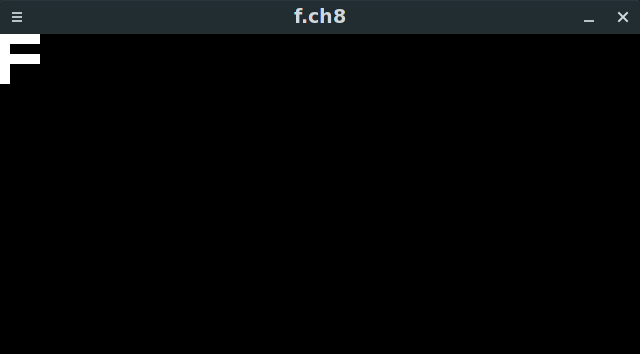
And here we launch it…
In the figure above you can see a simple program that draws a single digit F to the screen. This is a tiny program consisting of mere 10 bytes of code. It has 5 CHIP-8 instructions. How do I know it? Because every instruction is 2 bytes long!
The first instruction is 0xA04B. The second one is 0x6000. We will see what they do when we get to the instruction part of the tutorial. For now all you need to know is that the processor recognizes around 35 instructions and each one has a fixed size of 2 bytes.
Processor
The CHIP-8 processor works in the following way.
Read the value of a special PC register.
Fetch an instruction (2 bytes) from the RAM at the offset (aka address) PC.
Move PC to the next operation 2 bytes forward (PC := PC +2).
Execute the command encoded by the instruction we fetched on step 2.
Repeat step 1.
(Optional) Crash if instruction is invalid.
This cycle repeats itself until you halt the machine or it encounters an error instruction (unknown command encoded by those 2 bytes).
But wait, what is a register? A register is a very small named variable built into the processor. It has a fixed name and a size. CHIP-8 has:
CHIP-8 processor registers (and stack)
16 general purpose (meaning that you have a direct access to them as a programmer) 8-bit registers called V0, V1, …, V9, Va, Vb, Vc, Vd, Ve and Vf
16-bit general purpose register I – we use it to store addresses
8-bit special register DT – delay timer
8-bit special register ST – sound timer
16-bit pseudo register PC – program counter
8-bit pseudo register SP – stack pointer (more on this later)
You can use V0 and its friends to add numbers, read values from the RAM, store offsets and many-many other applications. You will learn more about them when we get to the instructions.
A processor also has 2 very special registers – PC and SP. PC (program counter aka instruction pointer) is storing the offset (aka address) of the next instruction. Next processor cycle will read and execute whatever operation is stored in the RAM at this location. It has to be at least 12 bits in size because the largest offset in a CHIP-8 program is 0x0FFF – 1 byte and a nibble in size. But since we don’t want to slice a byte, it is a 16-bit, or 2 bytes, register. Its upper half-byte is unused.
SP is a Stack Pointer. It is pointing at the top of the stack and it is an 8-bit register. But what is a stack? It is a fixed size storage that grows in one direction. You can put a value on top of the stack. You cannot access values below the top value unless you pop all items lying on top of the desired value.
Stack can push and pop a value
Usually stack is located in the RAM, the same RAM we are using for our program. But CHIP-8 has a separate stack memory space, so you cannot access it directly. It has 16 slots, 2 bytes each, and grows 2 bytes at a time. If stack size is at its limit, the top of the stack overflows to 0 and overwrites whatever value we had there. Of course, this is dangerous and can lead to some peculiar bugs.
Stack Overflow
Now let’s discuss one important application of the stack – function calls aka subroutines. At the start of the program stack is empty and SP is set to 0. When we call a subroutine in our game, CHIP-8 will push our current PC value onto the stack and increase SP by 1. It also sets PC to the address of the function we are calling. If we call one more subroutine, it will push our current PC onto the stack again, setting SP to 2. When we return from the subroutine, CHIP-8 takes whatever is at the top of the stack and sets PC to this value, decreasing SP by 1 afterwards.
Function Calls
Okay, that’s a lot of information, how much more there is to it? Thankfully not too much 🙂
Keyboard
Let’s blast through the keyboard first. CHIP-8 assumes that your keyboard looks something like this:
CHIP-8 keyboard binds 16 keys to a … peculiar layout
All we have to do is to bind part of our keyboard to this virtual keyboard just as on the figure above.
CHIP-8 can (but doesn’t have to) halt execution until a key is pressed. It then stores a key code to the processor register and continues executing our program.
Graphics
CHIP-8 also assumes that you have a display. It has a whooping resolution of 64×32 pixels. Pixels flow from LEFT to RIGHT, from TOP to BOTTOM. Every pixel has 2 colors. We will choose a classic white and black palette.
But you don’t just draw one pixel at a time. That would be too tedious. Instead you draw a sprite. What is a sprite exactly? It’s an image 8 pixels wide and X pixels tall. X is a number between 1 (1 row of 8 pixels) and 15 (15 rows of 8 pixels). Each bit of the sprite represents 1 pixel. For example, 0x87F0, or 1000 0111 1111 0000, is a sprite that is 8 pixels wide and 2 pixel tall. Its first pixel is white followed by 4 black pixels followed by 3 white pixels. It then switches to a lower row with 4 white pixels and 4 black pixels.
Sprite 0x87F0
All sprites are in the ROM, coexisting with the game code. This means that during execution we are storing our sprites in the virtual RAM. One curious implication is that you can accidentally draw an instruction instead of a sprite, producing garbage on the screen. CHIP-8 cannot distinguish sprite from an instruction, so it won’t crash the program.
Remember our scheme of the memory layout from way before? CHIP-8 VM reserves first 80 bytes for the hexadecimal digit sprites, 0 through F. Each sprite is 8 pixels wide (as any sprite) and 5 pixels tall, so each one takes 5 bytes of memory. We have 16 of them, so they take 16×5=80 bytes total of our RAM.
Standard digit sprites
There is an instruction to draw a sprite to a screen. You give it an X and Y offset on the display, an address of the sprite and its length and it draws it onto the screen. If it doesn’t fit, the remainder overflows to the opposite side of the display.
CHIP-8 is drawing sprites in a peculiar way. It is not blindly overwriting the pixel on the display. It is applying XOR (eXclusive OR) bit-wise operation on the display pixel and a spite pixel. Here what it looks like:
Sprite (top) XOR display (bottom)
Okay, we are almost at the end!
Other Components
CHIP-8 can also play music! Nah, I’m just kidding, it can beep in one sound for a while. You can make it beep by executing a special instruction that sets up a timer register ST. VM is decreasing its value at the rate of 60Hz. This is a fancy way of saying that ST is decreasing its value 60 times every second until it is equal to 0. CHIP-8 will beep for as long as ST value is not 0.
CHIP-8 also has a DT timer register that works essentially the same. However it is not tied to a sound. And you can access its value using – you guessed it – a CHIP-8 instruction.
CHIP-8 can also generate random numbers. There are no specifics, so any RNG will do. I personally use this one from the GDC talk because it is easier to use with unit tests.
And this is all that CHIP-8 has to it. It’s just a processor that can address up to 4KB of data. It has 16 8-bit general purpose registers, one 16 bit register for storing addresses, a program counter PC, a 16 byte stack, a display, a beeper, a keyboard and 2 timers. To run a CHIP-8 program you have to implement (aka emulate) every component.
Congratulations on making this far! You have done the trickier part of writing an emulator – understanding what the heck to do! Emulation is a very challenging problem, but also a very rewarding one. You essentially learn how computers work by implementing one yourself!
Please let me know if you find this post useful. If it gets enough attention I can make a follow-up CHIP-8 emulator tutorial where we implement it. Until next time!
Welcome back. This time we’re covering a cool feature of GNU/Linux called eBPF. It’s a set of tools that let you write small (or not so small) programs that run in the Linux Kernel whenever an interesting event happens.
In this post we will briefly discuss why BPF is useful. We will write a toy application that maintains a count of the opened file descriptors for all user processes. We’ll load a BPF application into the kernel, and get our data out of it.
By the way, BPF stands for Berkeley Packet Filter. Modern eBPF can do much more than packet filtering, but the name stuck.
You need to know a bit of C to follow along. If you know C++/Java/C#, you’re 65% there.
Let’s start with the basics. What is a Linux Kernel? To answer this question, let’s ask a more practical question – why does it matter to you?
In OS development there is a concept of kernel space and user space. In some way it resembles a superuser and a regular user concept. You can do whatever you want in the kernel space – including physical access to the hardware, filesystem manipulation, and memory allocations for the processes. This also means that if you have a bug in the kernel application (like a null pointer dereference), it will bring down your entire OS. Remember BSODs in Windows? That’s what happens when the kernel “panics”.
For this reason (and many-many others) modern OSes try to delegate as much of the functionality as possible to the “user space” applications. When you read “user space”, think of Node.js, Python, Firefox etc. They don’t have direct access to the protected resources, and cannot bring down the entire OS even if they try to (or at least that’s the idea). You can SegFault your C++ application as much as you’d like, but you shouldn’t ever bring down the whole system along with it.
Any time you need to perform a privileged operation (e.g. read a file, send a TCP packet over the network, allocate another useless object in Python), you have to call a function in the kernel. It is typically done through a “system call” mechanism. We will not dwell too much into it. You just need to know that it’s an API that stops execution of the user space application, and hands it over to the kernel space. The kernel performs some useful work on behalf of the process, and then returns to the unprivileged user mode execution.
There’s a “wall” between the user space and the kernel space
That’s nice, but I still don’t understand what BPF is!
Fair enough, so here’s another question – what if you want to run a program in the kernel space instead of the user space? This can be useful if you need to monitor some kernel activity (e.g. inspect a network packet). What are your options?
Before BPF there were 2 ways to run custom code in the kernel – you either change the kernel (and persuade Linus Torvalds and co that it’s worth it), or you write a kernel module. Both options have significant downsides. The former option can take years to implement and distribute, and the latter comes with a steep learning curve, security risks, plus a constant fear of panicking the kernel. And you need to sign the module to make it work with Secure Boot.
BPF let’s you pick a third way. What if you could write a small C application that triggers on a system call inside of the kernel, and it’s guarantied to never crash the system? This is done by running a VM inside of the kernel. You compile the bytecode for the VM, run the validation step, and attach the program to the kernel. However, there is a catch. VM puts some limits on what you can do in the kernel. For instance, writes are very restricted.
What is this post about?
We’ll write an application that maintains a count of opened FD (file descriptors) per user process. We shall develop a BPF application that is triggered on the openat and close system calls, and shall store the count in a BPF map (kernel data structure for BPF programs). We shall write both kernel space and user space code to access and modify this map.
Disclaimer: this program won’t actually maintain an accurate count (there are more syscalls that can open FDs), and there is a better way to do it without BPF. But it should be a good starting point for learning BPF, so let’s pretend that it’s useful.
Impatient readers can access the full kernel space code here and user space code here.
What do I need to follow along?
You will need a reasonably modern Linux distribution that comes with kernel version 5.15 or newer. You’ll have to install a couple of packages and clone a git repo. That’s about it! (Click to expand terminal commands)
# print the kernel version, make sure it's >= 5.15
uname -r

# Ubuntu
apt install clang libelf1 libelf-dev zlib1g-dev

# Fedora
dnf install clang elfutils-libelf elfutils-libelf-devel zlib-devel

# clone the repo and init subrepos
git clone https://github.com/libbpf/libbpf-bootstrap.git
cd libbpf-bootstrap
git submodule init
git submodule update --init --recursive

# test if the project compiles on your system
cd examples/c
make bootstrap
sudo ./bootstrap
The BPF Program Development Cycle
Before we dive deep into the code, lets briefly discuss how BPF program is compiled and loaded into the kernel.
There are multiple ways to write BPF programs. In early days, there was only a thing called BCC. It is a set of Python and C tools that lets you compile BPF code on the fly. You write a Python script, embed the C BPF code into the script (it’s literally a string inside of the Python script), and BCC figures out the rest. As a downside, you have to bring along a special clang compiler capable of compiling BPF code, and that bloats the distribution package.
Over the years BPF development cycle got better, and today we can compile BPF program once and run it on any system (mostly). It is known as Co-Re (Compile Once, Run Everywhere). I strongly recommend reading about it after this tutorial. libbpf-bootstrap has been created to showcase Co-Re capabilities.
We shall use libbpf-bootstrap project to quickly hack together a BPF application. It takes care of the project dependencies and compilation. We’ll start by modifying the bootstrap application in the examples/cfolder.
Compilation sequence for the bootstrap application Green represents a binary file, blue is a source code, orange is a generated file
The git repo also provides the bpftool app and libbpf C library for our system. We will be compiling them from the source code when we run make bootstrap command in examples/c folder.
libbpf is a C library that let’s you attach and manipulate BPF program from the user space. Essentially it is a wrapper around the BPF system calls. Since BPF is running in the kernel, we must use syscalls to interact with it. By default, only the superuser can use BPF system calls (for security reasons), so we’ll have to run our example with sudo.
bpftool is a utility application that links BPF programs. It tailors your BPF binary code to work with your kernel (this is explained in the same Co-Re post). It also generates a BPF “skeleton” header file. Without it you’d have to call raw libbpf functions to load the program, initialize the memory maps, attach the BPF to the kernel, cleanup the app etc. Skeleton takes care of the boilerplate code by pre-generating structs and functions like bootstrap_bpf__open, bootstrap_bpf__load, bootstrap_bpf__destroy etc. You can find libbpf documentation here. Linux Kernel provides good manual pages too.
In this post we shall modify the bootstrap.bpf.c kernel space source code to count the FDs. Next we shall modify thebootstrap.c user space source code to poll the map and print the pid-count pairs. We shall compile the app with the make bootstrapcommand. Lastly, we shall run the program with sudo ./bootstrap.
You can also run sudo cat /sys/kernel/debug/tracing/trace_pipe from a new terminal window to get the output of the bpf_printk function.
Implementation
Kernel Space App
Open examples/c/bootstrap.bpf.c file in your favourite file editor. Delete everything, and paste this code.
// SPDX-License-Identifier: GPL-2.0 OR BSD-3-Clause
// include BPF helper functions
#include "vmlinux.h"
#include <bpf/bpf_helpers.h>
#include <bpf/bpf_tracing.h>
#include <bpf/bpf_core_read.h>
#include "bootstrap.h"

// obligatory license
char LICENSE[] SEC("license") = "Dual BSD/GPL";

// declare a BPF map
struct {
	__uint(type, BPF_MAP_TYPE_HASH);
	__uint(max_entries, 1<<16);
	__type(key, pid_t);
	__type(value, s32);
} fd_count SEC(".maps"); // SEC takes care of registering
                         // this BPF map in the kernel
This snippet declares the obligatory license (the code won’t compile without it, you can read more here), and, most importantly for us, declares the fd_count BPF map.
A BPF map is a kernel data structure that serves 2 purposes: it’s a persistent storage for the BPF kernel program, and it’s a window into the kernel space data for the user space application. You can share the same BPF map instance between multiple BPF programs too. There are a dozen of map types, but we’re just using the good old hash map (aka a dictionary) to store process id (pid) and an associated FD count pair.
Maps require you to declare the max size of the map, and types for the key and value. This is passed to the kernel so it can allocate enough memory for the data structure. We’re allocating 216 = 65536 key-map pairs, the key type is pid_t (it’s a 32 bit signed integer, or s32, in the kernel), and value type is s32. SEC() is a macro that puts BPF code to the correct section of the BPF binary object.
Unlike normal C program, BPF code does not have a main function. That’s because BPF is reactive: you are “subscribing” to the kernel events (like tracepoints, kprobes or uprobes), and write a callback function to “hook” into the event.
Sequence diagram for the BPF app
Let’s write our first BPF callback.
/**
 * @brief Increment the counter on open
 */
// SEC macro takes care of attaching this function
// to the kernel tracepoint.
// this function will trigger when open syscall is invoked
SEC("tracepoint/syscalls/sys_enter_open")
int tracepoint__syscalls__sys_enter_open(
        struct trace_event_raw_sys_enter *ctx) {
    // get the user space pid
	u64 id = bpf_get_current_pid_tgid();
	pid_t pid = id >> 32;

    // get the element from the BPF map
	void *elem = bpf_map_lookup_elem(&fd_count, &pid);
	s32 value = 0;
    // have we set the map value yet?
	if (elem) {
        // increment by 1
		value = *((s32 *)elem);
		value += 1;
	} else {
        // no, but we know it is at least 1
		value = 1;
	}
    // put the new value into the map
	bpf_map_update_elem(&fd_count, &pid, &value, BPF_ANY);
	return 0;
}
Code explanation (expandable).
Here the SEC("tracepoint...") macro declares a callback function tracepoint__syscalls__sys_enter_open. The name of the function is not important. This function will be called whenever the kernel is processing open syscall.
You can get a list of tracepoints for your system by running the perf list command. If in doubt, ask Google or ChatGPT.
The code is pretty straight-forward. We start by getting the pid (process id) of the calling user space process. You can read about tgids and pids here.
We proceed to get the stored FD count from the fd_count map using the bpf_map_lookup_elem function. It accepts a pointer to the map and a pointer pointing at the key value, pid in our case. We verify that the returned value exists, or if we got a NULL pointer. If it exists, we get the value by performing some standard C pointer shenanigans (converting the returned void pointer to s32 pointer and de-referencing it), and increment it by 1. If the value does not exist, we simply set it to 1. We conclude by storing the updated value using the bpf_map_update_elem function. BPF_ANY simply tells BPF to not care if the value existed or not at the time of the update.
If you’ve opened the openat(2) man page in the explanation section, you might have noticed that there are actually 2 syscalls that can open a file – open and openat. This means that we need to process openat syscall as well. Let’s create a helper function handle_open to reuse the BPF code.
/**
 * @brief Increment the fd_count by a given value
 * @param increment - add this value to the counter
 * (or set if there is no value)
 */
void handle_open(int increment) {
	u64 id = bpf_get_current_pid_tgid();
	pid_t pid = id >> 32;

	void *elem = bpf_map_lookup_elem(&fd_count, &pid);
	s32 value = 0;
	if (elem) {
		value = *((s32 *)elem);
		value += increment;
	} else {
		value = increment;
	}
	bpf_map_update_elem(&fd_count, &pid, &value, BPF_ANY);
}

/**
 * @brief Increment the counter on open
 */
SEC("tracepoint/syscalls/sys_enter_open")
int tracepoint__syscalls__sys_enter_open(
        struct trace_event_raw_sys_enter *ctx) {
	handle_open(1);
	return 0;
}

/**
 * @brief Increment the counter on openat
 * Please note that these 2 syscalls still unfortunately
 * do not cover ALL possible cases
 */
SEC("tracepoint/syscalls/sys_enter_openat")
int tracepoint__syscalls__sys_enter_openat(
        struct trace_event_raw_sys_enter *ctx) {
	handle_open(1);
	return 0;
}
Now we need to add handler for the close syscall. We can reuse handle_open function by setting the increment parameter to -1. I should have called this function something better, but oh well ¯\_(ツ)_/¯.
/**
 * @brief Decrement the counter on close
 */
SEC("tracepoint/syscalls/sys_enter_close")
int tracepoint__syscalls__sys_enter_close(
        struct trace_event_raw_sys_enter *ctx) {
	handle_open(-1);
	return 0;
}
Besides open and close, there are two more syscalls we need to cover. What happens when a process exits, and another process reuses its pid? We would maintain a stale counter from the previous process for the new one. This means that we need to reset our counter whenever a new process is created, and delete the old value when a process is destroyed.
We can cover these cases by hooking into the exec and exit syscalls.
/**
 * @brief Reset the fd count for a new process
 */
// note that the tracepoint is a bit different
SEC("tp/sched/sched_process_exec")
int handle_exec(
        struct trace_event_raw_sched_process_exec *ctx) {
	u64 id = bpf_get_current_pid_tgid();
	pid_t pid = id >> 32;

    // an estimate for stdin and stdout files
    // the process could have inherited more FDs from
    // the parent...
	s32 value = 2;
	bpf_map_update_elem(&fd_count, &pid, &value, BPF_ANY);

    // this function prints to the
    // "/sys/kernel/debug/tracing/trace_pipe" file
    bpf_printk("Process %d created\n", pid);
	return 0;
}

/**
 * Remove process from the map on exit
 */
SEC("tp/sched/sched_process_exit")
int handle_exit(
        struct trace_event_raw_sched_process_exec *ctx) {
	u64 id = bpf_get_current_pid_tgid();
	pid_t pid = id >> 32;

	bpf_map_delete_elem(&fd_count, &pid);

    // this function prints to the
    // "/sys/kernel/debug/tracing/trace_pipe" file
    bpf_printk("Process %d exited\n", pid);
	return 0;
}
Code explanation (expandable).
The code is self-explanatory. We set the FD count to 2 (an estimate for stdin and stdout files) for the new process, and we remove the pid from the map on exit.
We also print a debug string with bpf_printk. It works like a normal printf function, with the same formatting conventions. You can access the output by reading the /sys/kernel/debug/tracing/trace_pipe file.
Save the BPF source code file and compile it with make bootstrap. You should get compilation errors for the bootstrap.c because we haven’t modified the user space program yet. If you are stuck, you can find the full BPF code here.
User Space Loader
Let’s implement the second part of the BPF program, the user space loader app. Start by opening the examples/c/bootstrap.c source file and copying the code from here. Save the file and compile the app withmake bootstrap. This time the program should compile without any errors. Run it with sudo ./bootstrap.
You should get an output similar to this (expand).
// ... a lot of lines skipped here
// The format is <pid>:<process name> <#FDs>. This count is updated every 5 seconds.
58498:kworker/10:3-events 2
59280:systemd-nsresou 8
59281:systemd-userwor 8
59282:systemd-nsresou 8
59283:systemd-nsresou 8
59284:systemd-userwor 8
59285:systemd-nsresou 8
59286:systemd-userwor 8
59287:systemd-nsresou 8
59590:kworker/u97:0-ttm 2
60005:kworker/u97:2-ttm 2
60006:kworker/u97:3-ttm 2
60007:kworker/u97:5-ttm 2
60008:kworker/u97:6-ttm 2
60009:kworker/u97:7-ttm 2
60010:kworker/u97:8-ttm 2
60011:kworker/u97:9 2
60089:sudo 16
60090:fprintd 13
60144:systemd 32
60145:kworker/2:1 2
60147:(sd-pam) 11
60159:psimon 2
60164:sudo 17
60165:bootstrap 16
483 processes
While the program is running, open a new terminal and execute sudo cat /sys/kernel/debug/tracing/trace_pipe. You should get a stream of messages whenever a process is created or killed.
          podman-7335    [010] ...21  5264.431155: bpf_trace_printk: Process 7329 exited

     unix_chkpwd-7342    [010] ...21  5264.716742: bpf_trace_printk: Process 7342 created

     unix_chkpwd-7342    [010] ...21  5264.743541: bpf_trace_printk: Process 7342 exited

     unix_chkpwd-7343    [023] ...21  5264.744604: bpf_trace_printk: Process 7343 created

     unix_chkpwd-7343    [023] ...21  5264.745066: bpf_trace_printk: Process 7343 exited

           <...>-7345    [019] ...21  5264.769114: bpf_trace_printk: Process 7345 created
Let’s dive deep into the code starting with the main function.
// a bunch of includes...

// a pid-count pair...
struct {
	pid_t pid;
	int32_t cnt;
} typedef pid_cnt;

static const uint32_t SLEEP_SECONDS = 5;
// BPF program representation in user space. It is
// generated by the bpftool in the bootstrap.skel.h file
static struct bootstrap_bpf *skel;
// do we need to exit?
static volatile bool exiting = false;
// store pid-count pairs from BPF map into a user space
// array (done in a main loop code later on)
static pid_cnt pid_fd_count[1 << 16];

/**
 * @brief print libbpf log messages to stderr
 */
static int libbpf_print_fn(
    enum libbpf_print_level level,
    const char *format,
    va_list args)
{
	return 0;
	/* Uncomment to enable debug logging */
	// return vfprintf(stderr, format, args);
}

// more stuff here...

int main(int argc, char **argv)
{
	int err;

	/* Set up libbpf errors and debug info callback */
	libbpf_set_print(libbpf_print_fn);

	/* set exiting=true on CTRL-C to exit gracefully */
	signal(SIGINT, sig_handler);
	signal(SIGTERM, sig_handler);

    // and even more code here...
Code explanation (expandable).
libbpf functions follow the standard C library conventions. We return 0 for success and anything else for error. A special errno value (available by including <errno.h>) contains the last error. There are standard values for errno like EINVAL or ENOENT. Thankfully strerror function provides us a human readable error message that we can print to stderr.
libbpf maintainers are kind enough to also provide access to their log messages. We can hook into the log stream by providing a callback to the libbpf_set_print function. Use it to debug a failure in BPF application.
Next, we open, load and attach BPF code to the tracepoints. If you need to initialize the BPF global variables, do so between OPEN and LOAD steps. And if you need to initialize BPF map values (like we do), make sure to do it between LOAD and ATTACH steps.
A BPF app life cycle
/**
 * @brief Count the number of opened FD by reading /proc
 * @param fd_callback callback for performing an arbitrary
 * action on the per-process FD count
 */
int collect_fd_count(int (*fd_callback)(int pid, int cnt))
{
    // iterate over all processes in /proc folder
    // count files in /proc/<pid>/fd folder
    // call fd_callback(pid, count) function to process
    /// the pid-count pair
}

/**
 * @brief Callback for the collect_fd_count function.
 * Set the BPF map value.
 */
int set_bpf_counter(int pid, int cnt)
{
	return bpf_map__update_elem(
        skel->maps.fd_count,
        &pid,
        sizeof(pid),
        &cnt,
        sizeof(cnt),
        BPF_ANY);
}

// ... some code here

// back to the main function
	/* Load and verify BPF application */
	skel = bootstrap_bpf__open();
	if (!skel) {
		fprintf(stderr, "Failed to open and load BPF skeleton\n");
		return 1;
	}

    /* Load & verify BPF programs */
	err = bootstrap_bpf__load(skel);
	if (err) {
		fprintf(stderr, "Failed to load and verify BPF skeleton\n");
		goto cleanup;
	}

	/* Important: initialize your maps between load and attach! */
	if (collect_fd_count(set_bpf_counter) <= 0) {
		fprintf(stderr, "Failed to set initial BPF map values\n");
	}

	/* Attach tracepoints */
	err = bootstrap_bpf__attach(skel);
	if (err) {
		fprintf(stderr, "Failed to attach BPF skeleton\n");
		goto cleanup;
	}
Code explanation (expandable).
Our first BPF related code is the bootstrap_bpf__open() function. It lives in the bootstrap.skel.h file that is generated by the bpftool when we run make bootstrap. It is initializing the skel variable. skel is of type bootstrap_bpf , which is in the same generated header file. It provides a facade for the BPF kernel application. It also gives us a handle for the BPF map, skel->maps.fd_count.
We initialize the fd_count map using the collect_fd_count function to read the pid-count pairs from /procfilesystem (this is that better way to get the pid-count data). We modify the BPF map in the callback function set_bpf_counter using the bpf_map__update_elem libbpf function.
Finally, lets explore the main loop of the user space app.
	/* Main Loop */
    // exiting variable is set by the SIGTERM or SIGINT
    // signal callback function
	while (!exiting) {
		int cnt = 0;
		pid_t pid;
		pid_t next_pid;
		int32_t fd_cnt;

		printf("\n\nFD Count\n");
		/* Iterate over the BPF map keys */
        // NULL tells libbpf that we want to get the first
        // key in the map
		err = bpf_map__get_next_key(
            skel->maps.fd_count,
            NULL,
            &next_pid,
            sizeof(pid));
		while (!err) {
			pid = next_pid;
			/* Get the value of the current BPF key */
			if ((err = bpf_map__lookup_elem(
                    skel->maps.fd_count,
                    &pid,
                    sizeof(pid),
                    &fd_cnt,
                    sizeof(fd_cnt),
                    BPF_ANY))) {
				break;
			}
			pid_cnt result = { pid, fd_cnt };
			pid_fd_count[cnt++] = result;

            // continue the iteration
			err = bpf_map__get_next_key(
                skel->maps.fd_count,
                &pid,
                &next_pid,
                sizeof(pid));
		}
		/* We do expect ENOENT at the end of the iteration */
		if (err == -ENOENT) {
            // sort and print the pid-count pairs...
		} else {
			fprintf(stderr, "Error: %s\n", strerror(errno));
		}

		sleep(SLEEP_SECONDS);
	}
Here we’re accessing the values directly from the BPF Hash map. Not all maps provide this kind of access, but hash map is one of them. There are other ways to get data out of the BPF application, like pinning the BPF map to a /sys/fs/bpf/<map_name> file, or using ring buffers to send events to the user space application.
Code explanation (expandable).
Iterating over the BPF map is a somewhat cumbersome. We start by declaring pid, pid_next key variables, and fd_cnt value variable. They shall be passed by their address to the BPF functions so that that BPF can mutate them. Remember, in C every variable is passed by the value, so if you need to mutate the value, you pass a pointer to the variable as a parameter.
We initialize the iteration by calling the bpf_map__get_next_key(skel->maps.fd_count, NULL, &next_pid, sizeof(pid)) function. NULL pointer indicates that we want to get the first key. This function accepts the current key, and writes the next key to the next_pid value. It returns 0 for success and -ENOENT when we reach the last key.
In the while loop, we call bpf_map__lookup_elem to get the value for the pid key. We store the pid-count pair in the pid_fd_count array and call bpf_map__get_next_key again to get the next key (or get -ENOENT and exit the while loop).
After processing all keys, we sort the pid_fd_count array by pid value, print the pid-count pairs and sleep for 5 seconds. If there was any error, we print it here too.
When we exit the main loop, we clean up by destroying the BPF application and de-attaching from the kernel. It’s also a good time to close any FDs and deallocate memory.
And that’s about it! Not too bad, huh?
Conclusion
Congratulations, you have just developed a kernel application! And we have done so without a single kernel panic!
For the next steps, you can start by hooking into more tracepoints that create file descriptors:
syscalls:sys_enter_open (covered)
syscalls:sys_enter_openat (covered)
syscalls:sys_enter_dup
syscalls:sys_enter_dup2
syscalls:sys_enter_dup3
syscalls:sys_enter_socket
syscalls:sys_enter_accept
syscalls:sys_enter_accept4
syscalls:sys_enter_pipe
syscalls:sys_enter_pipe2
syscalls:sys_enter_fcntl – can create new FDs through F_DUPFD
You can add a BPF global variable to monitor a single PID. We haven’t touched upon this topic, but the original bootstrap code can give you a good idea on how to do this.
BPF can hook into more than just syscall tracepoints. If there’s a particular kernel function you want to observe, chances are you get use kprobe to execute on function enter and exit events.
I recommend exploring the libbpf-bootstrap repo for more ideas. It provides both C and Rust examples for very interesting stuff.
We have only explored one way to get data out of BPF, that is, directly accessing the hash map. bootstrap example shows another way – sending events to user space via ring buffers.
Check out these resources to learn more about BPF:
Do you like solving Data Structure & Algorithms problems during interviews?
If you’re like me the answer is hell no. I hated doing it at my school. I hated doing it at university. And, surprise-surprise, I hate it now.
But here’s the deal – to get an awesome job you need to get good at solving coding problems. You just have to learn how to solve these abstract, out of real life challenges.
Imagine Segment Tree & Linked List instead of Sin Cos Tan
Unlike my more talented peers I never liked these problems. Instead of programming cool stuff like games I had to spend ungodly amount of time studying boring crap like segment trees that I hardly use anywhere.
However to succeed at an interview you have to learn at least basic algorithms and data structures. And one of problem solving techniques you’ll want to learn is called Dynamic Programming (aka DP).
DP seemed to give me the most trouble. I spent a good few years collecting nuggets of wisdom from here and there before it finally clicked with me.
In this blog post I hope to give you the same ‘aha’ moment. I hope to shine light on what DP is and how to use it.
Let’s start with the first major hurdle I have with DP.
Dynamic Programming is a terrible name
What do you think of when you hear ‘Dynamic Programming’?
Dynamic Programming is Fun and Intuitive!
I will confess – I had no idea what I was about to learn. It looks like we will, umm, program something that’s changing as we code it? I dunno ¯\_(ツ)_/¯.
It’s often said that there are 2 big problems in programming – cache invalidation and naming things. Looks like we have failed the latter problem here.
Let me give you an alternative name for DP – Brute Force with Caching. Since we all are well respected Computer Scientists here we must acronymify it – BFwC.
Alright, what does this mean?
Basically we solve our problem by recursive brute force. If our problem happens to have a nice structure we can split it into smaller sub-problems (this is the ‘dynamic’ part of the dynamic programming). We keep going down until we hit a trivial base case. We start going up solving sub-problems and in the process caching and reusing these solutions (that’s the ‘programming’ part of the dynamic programming). And magically instead of taking exponential time our brute force solution takes polynomial times aka much less time!
This is all nice and dandy but you’re probably still scratching your head. Let’s get our hands dirty with a simple problem. You might have heard about it before.
Let’s compute Fibonacci Sequence
I know, it’s not the most exciting or practical problem out there. But did you know that solution to this problem is actually a DP algorithm? Bear with me for a few minutes because we’re about to unearth some fundamental knowledge here.
In case you forgot Fibonacci Sequence looks like this:
0, 1, 1, 2, 3, 5, 8, 13, 21, 34, 55, 89, 144 …
You start with two numbers, 0 and 1. After that your next number is a sum of the previous 2 numbers.
Let’s define F[0] = 0, F[1] = 1. Then for i = 2, 3, 4 … F[i] = F[i-1] + F[i-2].
How can we compute the n-th Fibonacci number?
Well, one of the ways would be to use the definition directly:
int F(int n) {
    if (n == 0) return 0;
    if (n == 1) return 1;
    return F(n-1) + F(n-2);
}
We have successfully split our problem into sub-problems – to compute F[n] we compute F[n-1] and F[n-2] first.
Let’s say that we want to compute F[5]. That’s easy, F[5] = F[4] + F[3]. Okay, but what are F[4] and F[3]? Well, F[4] = F[3] + F[2] and F[3] = F[2] + F[1]. Great, but this is not an answer yet. Do we know what F[2] and F[1] are? Well, F[2] = F[1] + F[0]. But we do know what F[1] and F[0] are – they are 1 and 0 by definition!
Here’s a visual representation of what we’ve just discovered.
Dependency tree for the 5th Fibonacci number. Notice how we compute F[3] and F[2] multiple times (marked by the red and blue circles)
This is a dependency tree for Fibonacci numbers. To compute F[5] we need F[4] and F[3]. To compute F[4] we need F[3] and F[2] and so on. Can you see how our final result is the sum of just F[1] and F[0]?
This is a huge drawback in our approach. Can you see how we’re expanding F[3] 2 times and F[2] 3 times? Doesn’t that seem wasteful? Why not save F[4], F[3] and F[2] after we have computed them?
// we will cache our values into an array
// -1 means that we haven't computed this value yet
int fib[6] = {0, 1, -1, -1, -1, -1};

int F(int n) {
    // have we already computed this value before?
    if (fib[n] > 0) return fib[n];

    // if no, compute fib[n] using the definition and cache it
    fib[n] = F(n-1) + F(n-2);
    return fib[n];
}

// after calling F(5) fib will look like this:
// fib = {0, 1, 1, 2, 3, 5};
Wow, look how empty it is now!
Here we compute F[2], F[3], F[4] and F[5] just once. We cache and reuse their values as needed. This means that we don’t expand our computation down to the base cases F[1] and F[0]. We have just truncated the number of computations by half!
Let’s take a step back and reiterate over what we’ve just accomplished. We have started with a recursive brute force solution – compute F[n-1] and F[n-2] and then add these values. We have noticed that we’re recomputing F[i] for i=1..n-1 many times all over again. That’s wasteful so we started saving values to an array. We have modified our code to lookup value in the array. If it’s there we take it, otherwise we compute the value and store it into the array.
Okay, now we’re ready for a more challenging problem. Don’t worry, it’s not that bad… yet 😉
Let’s climb some stairs
Here’s another fun practical problem for you. Let’s say that you want to climb a staircase. You can make 1 or 2 steps at a time. Every stair has a computer on it. To move to the next stair you need to solve A[n] coding problems. You can start from the 1st or the 2nd stair. Given array A what is the minimum number of problems you must solve to climb to the top of the Stairs of Fun?
If you’re an avid competitive programmer you’d climb every step of this staircase twice
I encourage you to solve the problem on picture by hand. Spoiler – the answer is nine.
Now that you’re back – how can we solve this problem for any staircase?
You might be tempted to take the best solution at each step and hope that it gives you the best global result. Here’s another staircase for you:
Greed is good!
We start at stair 1 because otherwise we would solve 5 problems. Next we make a big step to the 3rd stair skipping 5 problems, than a small step to the 4th and then we reach the top. We must solve 3+4+1=8 problems.
This is called a greedy approach and sadly it doesn’t work here:
But is greed good?
Here’s a better solution – if we start from the second stair we need to solve 5+1=6 problems. Moral of the story – don’t get too greedy solving coding problems 🙂
Where greediness fails DP prevails. So let’s try this DP thing.
The trick is to figure out a recursive formula, not too dissimilar to the Fibonacci one. How can we do that?
Let’s imagine that we’re standing on the k-th stair. How did we get there? Well, we either climbed 1 step from the k-1-th stair OR climbed 2 steps from the k-2-th stair.
How do we know which one to take? Why not compute the minimal number of problems we must solve to get from both k-1 and k-2 stairs to the k-th stair and then take the smaller value?
Let’s denote S[k] as the minimum number of problems we must solve to get to the k-th stair. Let’s assume we do know S[k-2] and S[k-1]. Than we must solve at least S[k-2] + A[k-2] problems if we chose to climb 2 steps from the k-2-th stair OR we must solve S[k-1] + A[k-1] problems if we chose to climb 1 stair from the k-1-th stair. We can compare these two values and take the smaller:
S[k] = min(S[k-2] + A[k-2], S[k-1] + A[k-1])
You might say that’s great and all but we don’t know S[k-1] or S[k-2] – how is this useful? Well, we can apply the same trick to S[k-1].
S[k-1] = min(S[k-2] + A[k-2], S[k-3] + A[k-3])
And we can figure S[k-2] value by the same formula. This is a recursive brute force solution we were looking for.
Take a moment and think about the base cases i.e. values on which the recursion ends. Our S[0] and S[1] values are these special cases. How many problems do you absolutely need to solve to get to the first or the second stair? Since we start on either we have not solved any problems yet – so both S[0] and S[1] are 0.
S[0] = S[1] = 0
Here’s what the code looks like:
// vector is a C++ array
int min_cost(vector<int> &A, int n) {
    if (n == 0 || n == 1) return 0;

    int stair1 = min_cost(A, n-1) + A[n-1];
    int stair2 = min_cost(A, n-2) + A[n-2];
    return min(stair1, stair2);
}
Attentive readers would notice that this code has the same problem as our naive Fibonacci implementation – we will expand both S[n-1] and S[n-2] independently until we hit S[0] and S[1]. This means we’ll recompute S[2], S[3], S[4] etc. over and over again. So why not cache S[n] value after we compute it?
int S[100] = {0, 0, -1};

// vector is a C++ array
int min_cost(vector<int> &A, int n) {
    if (n == 0 || n == 1) return 0;
    if (S[n] != -1) return S[n];

    int stair1 = min_cost(A, n-1) + A[n-1];
    int stair2 = min_cost(A, n-2) + A[n-2];
    S[n] = min(stair1, stair2);
    return S[n];
}
To find an answer for any array A of size n you’d need to call min_cost(A, n+1). Why n+1? That’s because our staircase actually has n+1 stairs and the last stair (the ‘level stair’) has no cost. Take a look at the picture at the start of this section again. Yeah, it’s kind of weird, but that’s the how the problem was defined okay?
Top-Down vs Bottom-Up
Have you noticed that so far we’ve been writing recursive functions to solve our problems? This approach is called Top-Down.
There is an alternative way to code these solutions. Functionally they are the same – it’s up to you which one to use.
Bottom-Up solution starts from the base cases and works its way up to the top. Most of the time this means that we forgo recursive functions and start writing for loops.
How do we do this? For our staircase problem that’s as simple as looping over all array elements and filling S values starting from S[2]:
int min_cost_bt(vector<int> &A) {
    int n = A.size();
    vector<int> S(n+1, 0); // create an array with n+1 values
    // base cases
    S[0] = S[1] = 0;
    for (int i=2; i<=n; ++i) {
        stair1 = S[i-1] + A[i-1];
        stair2 = S[i-2] + A[i-2];
        S[i] = min(stair1, stair2);
    }

    // remember, we actually want to get to the n+1-th stair
    return S[n];
}
Some of you might be screaming at the monitor that we’re wasting a lot of memory here. Yes, we can just store the last 2 values and compute the answer, but that’s usually not the case. And my goal is to teach you DP, not memory frugality.
Bottom-Up solutions tend to run faster because you’re using loops instead of recursion. And recursion is always slower*.
*Not always, your millage might wary.
What problems can be solved by DP?
This is all well and good but how can you tell that the problem can be solved by DP? Sadly there are only 2 ways to know it – experience or trial-and-error.
However there are some rules of thumb that I can share with you. Take a look at the leetcode’s catalog of DP problems. Can you see how most of them ask you to find a min or max value (aka they are optimization problems)?
Another giveaway is the problem’s structure. I usually try to solve a problem by hand for the first few cases. If I happen to constantly reuse previous solutions (or some parts of the solution) it’s a flag that DP might work here.
More formally DP solutions are applicable to your problem if it has the following 2 properties.
Optimal substructure – you can solve it by a recursive formula.
Overlapping sub-problems – you need to compute sub-problems multiple times and they overlap – it makes sense to cache the values.
So where do I go from here?
I hope you are not afraid of the dreaded Dynamic Programming technique anymore. As you can see it’s actually just a brute force with caching.
I encourage you to solve a few easy DP leetcode problems. Try solving them on paper, then code Top-Down solution and then code a Bottom-Up solution. After that you’ll be ready for more challenging problems down the line.
In this chapter we will step away from our Raymarcher renderer. Instead we are going to implement a camera movement. We will be able to move forward, strafe, fly and look around using our mouse and keyboard.
This chapter is Godot-heavy. I assume you have some passing experience with the modern game engines (not Godot specifically). This means that I will not explain you what a script is. But I will guide you step-by-step on what to do.
Godot uses GDScript programming language for scripting. It is a Python-like language, very simple to learn and use. If you are not familliar with it, don’t worry. You will learn it by the end of this tutorial – it is that simple!
Actions
We will bind WASD keyboard keys for the basic movement and QE to move up and down. We could poll these keys directly (KEY_W, KEY_S, …). But there is a better way to do it. We will use Godot actions instead. Actions allow us to bind multiple inputs (like keyboard keys, mouse buttons, gamepad axis) to the same ‘action’. In the script we can ask Godot whether some action was triggered or not.
Open your project and go to Project -> Project Settings -> Input Map tab. You will see a list of existing actions. Add 6 more actions
camera_left
camera_right
camera_forward
camera_backward
camera_up
camera_down.
Here is my configuration:
Rotating the Camera around
Lets create a script that will move and rotate our camera around. I like to use many small scripts instead of a one large blob of code. So I created a subnode CameraMovement and attached a script to it.
Do not change any parameters when you create a script – just press Create button. A script file with code will appear. Delete everything except the extends Node line.
I took ideas from the Godot FPS Tutorial and LearnOpengl.com post. You can follow along this post and later read those articles to understand a theory behind our code.
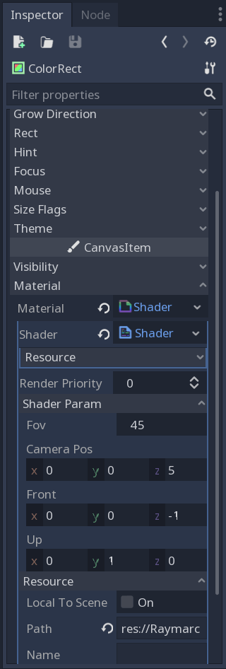
But before we start, select the ColorRect node and set the cameraPos parameter of our ColorRect shader to the (-3, 0, 0) and the front vector to the (1, 0, 0).
Don’t do it and all you will see is the black void instead of a sphere…
First we will define script variables. Enter the code below:
extends Node

# expose variables to the editor (and other scripts)
export(float) var MOUSE_SENSITIVITY = 0.05

# private variables
var mouse_offsets: Vector2 = Vector2() # in degrees
mouse_offsets store the pitch (x attribute) and yaw (y attribute) angles. We will update them as we move the mouse. Please note that we store angles in degrees.
Next add the following function:
func compute_direction(pitch_rad, yaw_rad):
    """
    Get front unit vector from the pitch and yaw angles
    """
    return Vector3(
        cos(pitch_rad) * cos(yaw_rad),
        sin(pitch_rad),
        cos(pitch_rad) * sin(yaw_rad)
    )
compute_direction converts our yaw and pitch angles into a front vector. To understand what is going on please follow this link.
Now add the _input(event)function. This is a callback function for the Godot. It is called when some event occurs. Events include:
Keyboard key was pressed or released
Mouse button was pressed
Mouse has moved
Action was triggered
Type in the following code:
func _input(event):
# update the pitch and yaw angles
    # intercept the mouse motion event and ignore all the others
    if event is InputEventMouseMotion:
        mouse_offsets += event.relative * MOUSE_SENSITIVITY
        # keep pitch in (-90, 90) degrees range to prevent reversing the camera
        mouse_offsets.y = clamp(mouse_offsets.y, -87.0, 87.0)
        var new_direction = compute_direction(
            deg2rad(-mouse_offsets.y),
            deg2rad(mouse_offsets.x)
        )

        # update front vector in the shader
        var color_rect = get_parent()
        color_rect.material.set_shader_param("front", new_direction)
First of all we check what is the type of our new event. We want to process the InputEventMouseMotionevent. It occurs when we move the mouse.
Then we check how far the mouse moved (event.relative) and scale it down. Then we make sure that the pitch angle is in the [-87, 87] degree range. If we fail to do so we will see the world upside down when we have moved mouse up too much.
We are computing new front direction using our utility function compute_direction and pass it to the shader.
Save the script and run the application. Move the mouse (or trackpad) around. You should get a smooth camera rotation, just like in the FPS games.
Pro tip: if you are using a laptop, plug it in. Otherwise the movement might be choppy.
However, there is an inconvenience: when you move mouse outside of the app borders you can no longer move the camera. Lets fix this issue.
Godot provides a few mouse modes. We are interested in MOUSE_MODE_CAPTURED and MOUSE_MODE_VISIBLE. The later is a default mode. We want to change that. Add the following function:
func _ready():
    # we want to capture the mouse cursor at the start of the app
    Input.set_mouse_mode(Input.MOUSE_MODE_CAPTURED)
_ready() is yet another callback function. It is called when the script starts running.
But what if we do want the mouse to leave our app? Lets toggle the mouse mode on the ui_cancel action. By default it is bound to the Escape key.
In the _input function replace
if event is InputEventMouseMotion:
with
if event is InputEventMouseMotion and Input.get_mouse_mode() == Input.MOUSE_MODE_CAPTURED
Append the following code to the _input function:
func _input(event):
    ...

    # capture/release mouse cursor on the 'Escape' button
    if event.is_action_pressed("ui_cancel"):
        if Input.get_mouse_mode() == Input.MOUSE_MODE_CAPTURED:
            Input.set_mouse_mode(Input.MOUSE_MODE_VISIBLE)
        else:
            Input.set_mouse_mode(Input.MOUSE_MODE_CAPTURED)
Save and run. Now the mouse should not be visible and it should not leave the borders of our app. Hit Escape on your keyboard and the mouse cursor will appear. Hit it again and you will regain control of the camera. Perfect!
If it is not perfect, check out my GitHub project. git checkout part3-rotation will do the trick.
Moving the Camera
Now lets utilize the keyboard to move around our world. Add 2 more helper functions to the CameraMovement script:
func compute_direction_forward(yaw_rad):
    """
    Get front unit direction on the XZ plane (do not cosidering the height)
    """
    return Vector3(
        cos(yaw_rad),
        0,
        sin(yaw_rad)
    )


func compute_direction_right(yaw_rad):
    """
    Get right unit direction on the XZ plane (do not cosidering the height)
    """
    return Vector3(
        -sin(yaw_rad),
        0,
        cos(yaw_rad)
    )
We want to obtain the ‘forward’ and the ‘right’ relative directions. All we need is the yaw angle.
Note where are the x and z axis
Lets rename forward as d. Than we can obtain the projections of d on the x and z axis using our yaw angle:
|d| is the length of d
If we move ‘forward’ (in the direction of d) 1 unit ahead, we move (1 * cos(yaw)) on the x axis and (1 * sin(yaw)) on the z axis. That’s where the cos and sin come from in our helper functions. Note that we leave y coordinate alone – we don’t want to fly up or down when we are running!
‘Right’ direction (it is orthogonal to the ‘forward’) is obtained through the following fact: if you have a 2d vector (a, b), then the vector (-b, a) is orthogonal to it.
Let’s implement this idea in our code. Add MAX_SPEED and velocity variables to the script:
# expose variables to the editor (and other scripts)
export(float) var MOUSE_SENSITIVITY = 0.05
export(float) var MAX_SPEED = 300

# private variables
var velocity: Vector3 = Vector3()
var mouse_offsets: Vector2 = Vector2() # in degrees
Add yet another helper function:
func update_velocity(delta):
    """
    Update velocity vector using actions (keyboard or gamepad axis)
    """
    # get current step size
    var delta_step = MAX_SPEED * delta
    var direction_forward = compute_direction_forward(deg2rad(mouse_offsets.x))
    var direction_right = compute_direction_right(deg2rad(mouse_offsets.x))
    # we will have no intertion
    # if we release buttons, we will stop immediately
    self.velocity = Vector3()

    ...
delta is the time (in seconds) since the last update. Long story short – you have to scale the step to make movement consitent across different computers (or consoles).
Lets process the camera_forward and camera_backward events:
Lets update cameraPos shader variable in separate function:
func update_camera_position(delta):
    """
    Update camera position and pass it to the shader
    """
    var color_rect = get_parent()
    var cur_pos = color_rect.material.get_shader_param("cameraPos")
    var new_pos = cur_pos + self.velocity * delta
    color_rect.material.set_shader_param("cameraPos", new_pos)
And use the Godot’s _process_physics callback to actually obtaint movement:
func _physics_process(delta):
    """
    Move the camera with the steady 60 FPS loopback
    """
    update_velocity(delta)
    update_camera_position(delta)
Save the script and run the app. Press WASD to move around and QE to elevate the camera.
In case you are stuck, git checkout part3-movement.
Bonus: Field of View
And while we are at it, lets add zooming with the mouse wheel! Add another child to the ColorRect node and name it Fov. Attach a script to it.
Add 2 more actions. Go to the Project -> Project Settings -> Input Map tab and add camera_zoom_in and camera_zoom_out actions. Bind the Wheel Up and Wheel Down mouse buttons to them, respectively.
Edit the Fov.gd script. Type in the following code:
extends Node

export(float) var WHEEL_STEP = 4

# onready will execute when the script is starting to run
onready var fov = get_parent().material.get_shader_param("fov")

func update_fov(new_fov):
    # keep FOV in the [15, 135] range
    self.fov = clamp(new_fov, 15, 135)
    get_parent().material.set_shader_param("fov", self.fov)

func _input(event):
    """
    Process the mouse wheel scroll event to change the FOV
    """
    # intercept the mouse wheel up/down event
    if event.is_action_pressed("camera_zoom_in"):
        update_fov(fov - WHEEL_STEP)
    elif event.is_action_pressed("camera_zoom_out"):
        update_fov(fov + WHEEL_STEP)
Save and run the app. Try scrolling the mouse wheel (or panning on a touchpad). You should observe zooming effect.
If you are stuck, git checkout part3-fov to get the full project.
sdf is our main function. It tells us how far the point pos is from the scene. sdSphere is a SDF for a sphere. We pass it our position p, centre of the sphere c and its radius r.
As you can see, it is a very simple algorithm. We march along the ray at most MAX_STEPS times. We use ray equation
t is a number, origin and direction are vectors. directionis a unit vector
to compute current position in space. We use sdf to check if we have hit an object. If we have, we return return white color, otherwise march along the ray again. If we have not hit the ray in MAX_STEPS steps, we return black color.
Lets use this function in our main shader function:
uniform int MAX_STEPS = 250; // march at most 250 times
uniform float MAX_DIST = 20; // don't continue if depth if larger than 20
uniform float MIN_HIT_DIST = 0.00001; // hit depth threshold
Save the shader and run application. You should see white circle on a black background like here:
If you are stuck, you can use my project on GitHub. git checkout part2-unshaded will do the trick.
Phong Lightning Model
Basic Idea
All we can see now is a white circle on a black background. You might even think that our sphere isn’t spacial at all! And you are somewhat right – without the lights our scene looks flat. We need to implement a light model in order for the sphere to appear volumetric.
We will implement Phong light model. It states that the illumination of an objectconsists of the 3 parts
Ambient component – no scene is completely black.
Diffuse component – dirrect impact of the light.
Specular component – glossiness of an object.
To gain better intuition, check out this link: LearnOpengl, Basic Lighting. On Wikipedia you can find formula we will be using in this tutorial:
Scary but in the end it all comes down to the 3 bullet points:
Pixel color is deternined by the sum of the 2 components:
Ambient lightning, uniform for every object on the scene.
Sum of contributions of all light sources
Each light source contribution is a sum of 2 parts:
The diffuse lightning – simulates the directional impact a light has on an object.
The specular lightning – simulates the bright spot of a light that appears on shiny objects.
Now, we have to discuss the normal vector of a surface. What is it and why should you bother? Well, normal to a surface at some point is a unit vector that is orthogonal to the surface at that specific point:
You need this vector in order to compute the diffuse lightning contribution. Lets say the a we have a toLight and a normal vectors. toLight is a unit vector from the hit point to the light source position:
Because toLight and normal are unit vectors, their dot product is equal to a cosine of an angle between the vectors:
||v|| is a length of a vector v
The more toLight and normal are aligned in the same direction, the stronger light reflects from the surface. The contribution cannot be negative, so if cosine is negative we set the contibution to 0.
How do we compute the normal to a surface? Well, the normal vector is equal to a nomalized gradient of a SDF at given point. Gradient is a vector that tells us how fast the function grows in small change of its parameters. Feel free to read more about it here. All you need to know for now is that it can be approximated using nothing but SDF itself.
Specular Component
Finally, we want to compute the specular lightning contribution. It is computed by the following formula:
Lets implement the Phong model in our shader! First of all lets define some uniform variables:
uniform float globalAmbient = 0.1; // how strong is the ambient lightning
uniform float globalDiffuse = 1.0; // how strong is the diffuse lightning
uniform float globalSpecular = 1.0; // how strong is the specular lightning
uniform float globalSpecularExponent = 64.0; // how focused is the shiny spot
uniform vec3 lightPos = vec3(-2.0, 5.0, 3.0); // position of the light source
uniform vec3 lightColor = vec3(0.9, 0.9, 0.68); // color of the light source
uniform vec3 ambientColor = vec3(1.0, 1.0, 1.0); // ambient color
We need to compute normal vector to the surface we have hit. Here is the function:
We check how SDF changes when we change X, Y and Z coordinates by a small amount (arount 0.0001). For X, we compute SDF in points (X+0.0001, Y, Z) and (X00.0001, Y, Z) and subtract these values. We repeat this for Y and Z. Then we normalize the resulting vector.
We are ready to implement Phong model. Here is my function:
vec3 blinnPhong(vec3 position, // hit point
                vec3 lightPosition, // position of the light source
                vec3 ambientCol, // ambient color
                vec3 lightCol, // light source color
                float ambientCoeff, // scale ambient contribution
                float diffuseCoeff, // scale diffuse contribution
                float specularCoeff, // scale specular contribution
                float specularExponent // how focused should the shiny spot be
)
{
    vec3 normal = estimateNormal(position);
    vec3 toEye = normalize(cameraPos - position);
    vec3 toLight = normalize(lightPosition - position);
    vec3 reflection = reflect(-toLight, normal);

    vec3 ambientFactor = ambientCol * ambientCoeff;
    vec3 diffuseFactor = diffuseCoeff * lightCol * max(0.0, dot(normal, toLight));
    vec3 specularFactor = lightCol * pow(max(0.0, dot(toEye, reflection)), specularExponent)
                     * specularCoeff;

    return ambientFactor + diffuseFactor + specularFactor;
}
Then we modify our raymarch function to return computed illumination color instead of plain white:
/* before change
...
if (dist < MIN_HIT_DIST) {
    return hitColor;
}
...
/*

/* after change */
if (dist < MIN_HIT_DIST) {
    return blinnPhong(pos, lightPos, ambientColor, lightColor,
           globalAmbient, globalDiffuse, globalSpecular, globalSpecularExponent);
}
Thats all the changes! Save the shader and run an application. You should see the same picture:
If you struggle, please feel free to use my GitHub project. git checkout part2-shaded should get you here.
With some parameter tweaking you can get the following result:
That is it for now! There is a lot more to cover but that’s as far as I am willing to go right now. You can continue exploring Raymarching from the Jemie Wong’s excellent blog. Cheers!
In the previous chapter we have set up a sandbox Godot project. We have created a fullscreen shader and have used it to display an opaque red color. Quite boring.
In this chapter I will cover basics of Raymarching. I will provide you a very brief explanation of the technique and focus on implementing camera in the shader. You can jump to the code first and than see the explanation or vice versa.
Theory
Raymarching overview
Lets consider our real world. How do we see things around us? Light sources produce light. Light moves along the ray until it hits some object. Eventually it is either consumed by the object, reflected away from it or refracted. Either way, this beam of light somehow reaches your eye (or camera lens).
We can see objects because the light is reflected back to our eye. Without the light source we can see no objects.
We are going to simulate this phenomenon. But instead of tracing millions of rays from all the light sources (of which very few would hit the eye) we will do the opposite. We will shoot our rays from the eye and see what they hit. Than we will determine pixel color using the hit point, properties of the light source and of the object.
Stolen from the Nvidia website
Now comes the tricky part. How do we know what our ray hits along its path? Well, we could:
For each object find the intesection point with one ray at a time. We are going to pick the one closest to an eye. This is the raytracing technique. If we have N objects and R rays than we have to perform N*M collision tests at worst.
Move along the ray with some steps and check whether or not we have hit some object. This is the raymarching technique.
Okay, so we are going with the second approach. You might ask “How do I pick a step?” and “How do I know that I have hit the object”? And here comes the brilliant solution.
Meet the SDF – Signed Distance Function (takes vec3 -> produces float). It accepts a point in space and tells how far away are we from the objects on the scene.
Here is an example: lets say we have 1 sphere. It is centered in (0, 0, 0) and its radius is 1. Now lets say that we have point (2, 0, 0). How far away are we from the sphere? The answer is
R is a radius, subscript marks coordinate of the Sphere’s center
And in our example
The distance from the point (2, 0, 0) to the sphere is equal to 1
How can we answer on “How do I know that I have hit an object?” If SDF returns small value (ex. 0.0001) – you are very, very close to an object. So close that you can say neglect it. If at any point along the ray SDF returns very small number – our ray has hit an object on a scene.
Lets answer on “How do I pick a step?” If you pick a constant step (say 1 unit each time) you have 2 problems:
If you pick large step you are likely to overshoot your object.
If you pick small step you are moving very slowly and can miss the 60 FPS goal.
And SDF comes to a rescue again! Lets say that SDF has returned 4. What does it mean? It means that an object is at least 4 units away from your current position, no matter the direction you are facing. It can be further but never closer. So why not march in the direction of the ray 4 units forward?
Taken from the video below (2:49)
And here is full the answer: you move as far as the SDF tells you to. This way you will never overshoot the target and will move much, much quicker than with the small constant step.
Now, there is more stuff to consider. But this covers the essential basics. Please watch the video below (starting at 1:55) to gain even better intuition.
Camera
Camera is an object that has a position and a field of view. It represents our viewing window into the virtual world. My camera implementation is based on the video below.
We are going to calculate ray direction in our fragment shader and display it as a color.
First of all we need a set of parameters that control our shader:
uniform float fov = 45.0; // the vectical field of view (FOV) in degrees
uniform vec3 cameraPos = vec3(0.0, 0.0, 5.0); // position of the camera in world coordinates
uniform vec3 front = vec3(0.0, 0.0, -1.0); // where are we looking at
uniform vec3 up = vec3(0.0, 1.0, 0.0); // what we consider to be up
Uniform variables can be changed outside of the shader (either from script or the Inspector tab). Later on we can manipulate camera from the game engine using keyboard and mouse (or touch on phones and tablets).
For now we will be doing no raymarching yet. We will merely set up a camera. For each pixel we are going to compute a direction that the ray is traversing in.
In the fragment shader add a new function. It will accept the screen resolution and a location of a pixel in normalized coordinates (in range [0, 1]) and produce ray direction:
After that we convert uv (nomalized pixel coordinates) to a range [-1, 1] and invert the y coordinate (because in Godot Y axis flows from the top to the bottom). We can obtain the contribution of the up and right vector:
vec3 getRayDirection(vec2 resolution, vec2 uv)
{
    ...
    // convert coordinates from [0, 1] to [-1, 1]
    // and invert y axis to flow from bottom to top
    vec2 screenCoord = (uv - 0.5) * 2.0;
    screenCoord.x *= aspect;
    screenCoord.y = -screenCoord.y;

    // contibutions of the up and right vectors
    vec2 offsets = screenCoord * tan(fov2);
    ...
}
Now comes the interesting part. We compute the unit front, up and right vectors and make sure they are orthogonal to each other. This creates a coordinate frame. We use it to compute our ray direction. Don’t forget to normalize it!
And we have our ray direction! Now, to test how this works we will display the direction as a color. However, because the color components should to be in range [0, 1] and the coordinates of the direction are in [-1, 1] we have to do one more conversion. Here is the main fragment shader function:
...
void fragment()
{
    vec2 resolution = 1.0 / SCREEN_PIXEL_SIZE;

    vec3 rayDir = getRayDirection(resolution, UV);
    // convert ray coordinates from [-1, 1] range to the [0, 1]
    vec3 adjustedRayDir = (rayDir + 1.0) / 2.0;
    // show direction on screen as a color
    COLOR = vec4(adjustedRayDir, 1.0);
}
SCREEN_PIXEL_SIZE is a Godot constant I use to compute resolution. You can read more about it here.
Here is the full shader code:
shader_type canvas_item;

uniform float fov = 45.0;
uniform vec3 cameraPos = vec3(0.0, 0.0, 5.0);
uniform vec3 front = vec3(0.0, 0.0, -1.0);
uniform vec3 up = vec3(0.0, 1.0, 0.0);

vec3 getRayDirection(vec2 resolution, vec2 uv)
{
    float aspect = resolution.x / resolution.y;
    float fov2 = radians(fov) / 2.0;

    // convert coordinates from [0, 1] to [-1, 1]
    // and invert y axis to flow from bottom to top
    vec2 screenCoord = (uv - 0.5) * 2.0;
    screenCoord.x *= aspect;
    screenCoord.y = -screenCoord.y;

    // contibutions of the up and right vectors
    vec2 offsets = screenCoord * tan(fov2);

    // compute 3 orthogonal unit vectors
    vec3 rayFront = normalize(front);
    vec3 rayRight = cross(rayFront, normalize(up));
    vec3 rayUp = cross(rayRight, rayFront);
    vec3 rayDir = rayFront + rayRight * offsets.x + rayUp * offsets.y;

    return normalize(rayDir);
}

void fragment()
{
    vec2 resolution = 1.0 / SCREEN_PIXEL_SIZE;

    vec3 rayDir = getRayDirection(resolution, UV);
    // convert ray coordinates from [-1, 1] range to the [0, 1]
    vec3 adjustedRayDir = (rayDir + 1.0) / 2.0;
    // show direction on screen as a color
    COLOR = vec4(adjustedRayDir, 1.0);
}
Run the application. You should see the simillar result:
In any case, the full project is available at my GitHub repository. Just run git checkout part1 to get to this point.
Now, lets tweak parameters we defined on the beginning of the tutorial. Look at the shader parameters in the Inspector window:
Change the fov to 90 and front to the (0, 0, 1). Run the application. You should see similar result:
That’s it for now. A little boring, I know. In the next chapter we are finally going to draw some objects. Until then, cheers!
Raymarching is a rendering technique. It takes a 3d scene (bunch of objects like spheres, triangles, cubes, lights etc.) and produces a 2d image. Here is a list of common rendering techniques:
Rasterizer – for real-time rendering (games, 3d modeling, user interfaces…). Fast but not realistic. Complex effects are hacky (reflections, refraction, blending…).
Raytracer – for realistic images with reflections and refraction (Pixar cartoons, movies…). Very beautiful images, simple to implement (at least at basic level), trivial to parallel. However, it is quite inefficient and not suited for real-time rendering yet.
Raymarcher – quite similar to the raytracing. It makes a good usage of some very clever math tricks to speed up rendering. But don’t get me wrong – it is not a replacement for the raytracing! Simplicity, small executable sizes and ability to run concurrently makes it perfect for demos!
Static randering: you define a static scene with objects, light sources etc and render one single image.
Real-time rendering: your program constantly updates and renders scene (preferably at 60 FPS – Frames Per Second).
Goal of this Tutorial
I am going to teach you how to implement a real-time raymarcher using Godot game engine and a fragment shader. You will be able to interact with the scene, move the camera around and tweak the field of view (FOV).
There are many ways you could go with implementing a raymarcher. If you are hardcore, you can imlement everything yourself using some 3d graphics API (OpenGL, DirectX, Metal, Vulcan). If you want to start quickly, you could use ShaderToy (I have done so on my first try). But I would recommend using a game engine.
While most would go with Unreal or Unity, I’ve decided to give Godot a try. Now, don’t dismiss it right away. Godot has a lot of nice perks and features:
It is cross-platform (you can develop on Windows, Mac, Linux, Android, IOS)
It is completely free
It is open-source
You 100% own your project (with no legal BS)
It is quite simple
It is quite small (~50 MB executable)
Portable engine editor (no need to install it)
No registration required to download it
It is a mature project
Community is very active and helpful
Game engine allows you to create application once and build it for any platform it supports. Projects are portable, so you will not encounter irritating problems when you change your environment. And game engine makes adding new features a breeze.
Setup environment
Okay, enough talking, lets do some coding!
Download Godot and launch it. Add new project with the renderer set to “OpenGL ES 3.0”.
You should see a window like this…
Press on the “Custom Node” and search for the “Node” (with the grey doughnut icon) in the Scene tab.
Search for the “Node” and press “Create”
Right click on the “Node” and add a “Control” child.
Right click on the “Node” you have just added. Select “Add Child Node”. Search for the “Control” and press “Create”
Now select the Layout -> Full rect layout.
Right click on the “Control” node and add a “ColorRect” child. Select the Layout -> Full rect layout
It should look like this…
Loot at the Inspector on the right and open the “Material” property. Click on the “Material [empty]” and choose new “ShaderMaterial”. Click on the sphere that appeared.
Our ColorRect has a material but no Shader yet
Click on the “Shader [empty]” and choose “New Shader”. Click on the “Shader” An editor should appear on bottom of the screen.
Editor will only appear when you press on the Shader combobox just below the Material (with the Sphere image to the right of it)
Save the scene and name it Raymarcher.tscn. Run the project (right top corner or press F5). Select Raymarcher.tscn as a main Scene. If you see a red rectangle like on the image above – you have done well!
Otherwise feel free to clone my project from the GitHub. Use your terminal and type git checkout part0. You will get the same red rectangle as on the image above.
Conclusion
Thats it for now! We have set up a sandbox that will turn into a full-fledged application one day. Hopefully you are as hyped as I am to render your first scene!
Meanwhile you can visit the links below. You will find there my GitHub project, useful blogs and videos. I have used them myself to implement a Raymarcher. Cheers!